Attempt on getting smoother probabilistic distribution of ensemble climate prediction output produced by global climate models.

Background Part 1
Reflecting grave concern on the global environmental degradation relating probably to anthropogenic warming, the application of short-term climate information or seasonal prediction to various societal activities is now gathering momentum. After a decade of the world-leading short-term climate variability prediction studies, especially on the important tropical variability such as ENSO and IOD which exerts a tremendous societal impact on Asia-Oceania regions, JAMSTEC had launched application studies using the outcome of a state-of-the-art climate model SINTEX-F (Fig. 1).
This activity is in accord with the third world climate conference (WCC-3) high-level declaration on the establishment of a global framework for climate services and, so far, we have been promoting agricultural applications through collaborating with domestic as well as such international institutions as IRRI.
Fig.1: A schematic view of SINTEX-F model and an example of its ensemble prediction on IOD.
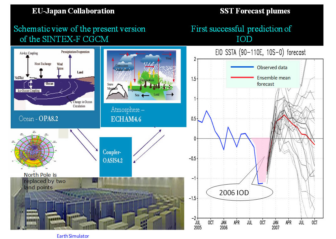
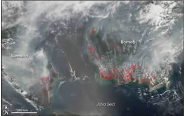
Fig. 2: Huge societal impact caused by 2006 IOD
Extreme Weather Conditions Associated with 2016 IOD
East African Flood (More than 1 million people have been uprooted in Kenya)

Indonesian Forest Fire
Australian Drought

State-of-the-art (short-term) climate predictions issued by the world-leading operational centers and JAMSTEC APL are the outcomes of sophisticated climate models (coupled atmosphere and ocean models) that run on super-computers equipped with huge data storage. Needless to say, for global climate studies and predictions, a global model is an inevitable research tool, however, from the view point of application studies, we can safely say that, in almost all cases, a set of time series data on (or around) a specified grid point, as is illustrated in the right panel of Fig. 1, are all we need for the studies. Totally independent of this aspect of application studies, as a part of cutting-edge research efforts in improving the quality of prediction by enhancing computing capability, considerable increase of ensemble members of climate models aiming at having better probabilistic distributions of climate variables is now in the planning stage.
Taking these two different aspects of the ongoing activities in climate study community into consideration, it seems to deserve considering a possibility that simulated ensemble outputs illustrated in Fig. 1 may be further refined (to have smoother probability density distribution) in a certain approximate sense by utilizing advanced knowledge on, say, filtering of statistical modeling, of which performance will be evaluated later by direct simulations with a larger number of ensemble.
The aim of studying such a possibility is clear. Obtaining smoother probabilistic distributions of climate variables even in an approximate sense without running costly super-computers is quite desirable from the view point of application studies as well as the dissemination of climate prediction output to general public.
Springboard for discussion and goal
As a speculative draft of such an attempt, I am going to provide a statistical model as a testbed of our discussion. The details of the model will be given later at the workshop. At present, here we describe a basic idea of the statistical model. We start from a simple fact that no further information is available other than ensemble time series data provided from a given climate model. To extract meaningful structural information from a given finite-length time series data without adding artificial information, we can employ the Maximum Entropy Method (MEM) by Burg. It can be shown that a give finite-length time series data can be approximated by a generalized trigonometric series whose frequencies are determined through MEM and the approximation is done in a least-square sense. That is to say, a given finite-length time series data is transformed into the sum of a generalized trigonometric series with suitable length (a deterministic part which contains the information on important climate mode in terms of frequencies) and a Gaussian noise term that may be interpreted as a simplified model of intrinsic chaotic behavior of climate.
Thus, for each ensemble member of the output of a given climate model, we can specify a “statistical sub-model” having a deterministic as well as a non-deterministic noise term which can be run as many times as we want. Simple addition or a collection of these sub-models leads to a targeted statistical model that would produce a smoother probabilistic distribution.
As the number of ensemble provided by a climate model increases, the difference between the original output of climate model and that of the transformed statistical model would converge, so that the above model could be a candidate of the targeted model. Of course, there would be other better ways to have such statistical models and the real challenge or goal is, if possible, to identify a measure to evaluate the performance of candidate models.
Background Part 2
In natural vegetation, a plant population is composed of individuals having various sizes (e.g. plant weight, plant height, and stem diameter) and competing with other individuals for resources such as light, nutrients, water and so on. To investigate how competition and coexistence processes emerge from such a complex system is one of the most interesting subjects in plant ecology. Furthermore, to investigate size-structure dynamics and species co- existence conditions in plant communities is important for applied biological sciences such as agriculture and forestry.
Many models so far proposed for the study of growth dynamics in plant populations divide into two categories, spatial and non-spatial models. Most of these models consider interactions between individuals based on the growth of each individual in a population. Spatial models take into account spatial distributions of individuals, whilst non-spatial models do not, assuming that the spatial distribution of individuals is homogeneous.
Further Background Information
Model
Let us consider an even-aged plant population which grows in a homogeneous environment, i.e. the plants have the same size distribution per unit area at any place in the stand we consider. Let f (t, x) be a distribution density of individuals of plant size x (e.g. plant weight, height and stem diameter) per unit area at time t. It is assumed that the basic equation governing the dynamics of f (t, x) is given by
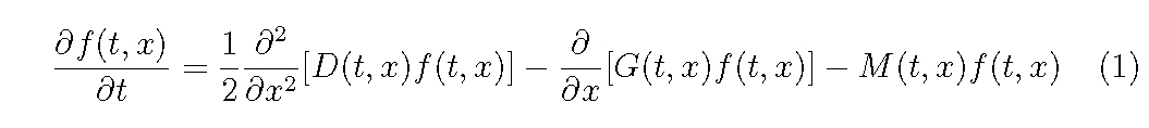
where G(t, x) and D(t, x) are the mean and variance of growth rate in plant size, x, respectively, and M (t, x) is the mortality rate. The diffusion term may be important for a long-term simulation in which the statistical variability of growth rate may largely affect the size distribution (Hara, 1984).
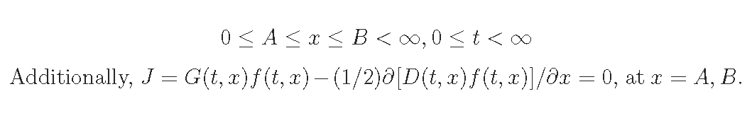
Here, we consider an even-aged plant population without the recruitment,
i.e. zero birth rate, then impose the boundary condition.

Self-thinning rule
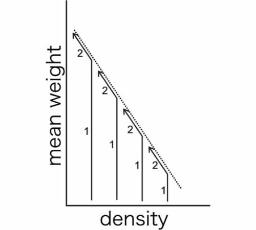
Yoda et al. (1963) proposed the so-called ’-3/2 power law of self-thinning’, which states that the relationship between mean plant weight, x ̄, and density, ρ, is given as

where K and c are constants and c ∼ −3/2 irrespective of species and conditions (see also Westoby, 1984; White, 1981).
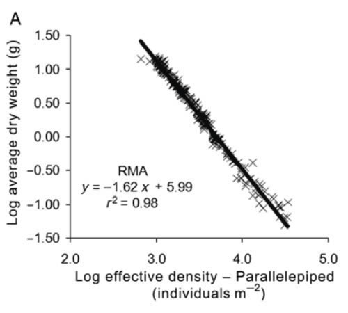
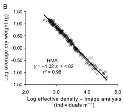
Dry weight of individual mussels vs culture density. and linear fits performed by RMA. where N is the effective density calculated from the projected area of the parallelepiped (A). and where N is the effective density calculated from the image analysis (8). In both cases. only RMA is shown because the SFF estimates identical parameters and the likelihood value is less than that obtained using RMA. ANCOVA following Zar (1984) was performed to compare the exponents observed in the present study with theoretical values for FST and SST (-4/ 3 and -3/2. respectively). https://academic.oup.com/mollus
Problem
From eq.(1), the density ρ(t) and the mean weight x ̄(t) are given as follows:

Let us assume the empirical D and G function forms, while several types of function forms are proposed and G function can be formulated theoretically based on canopy photosynthetic processes.
For D function,

For G function,

And for M function, as it should M (t, x) → 0 as x → ∞, we can assume
the function form as follows:

Then, are there some restrictions among functions, D,G, M and f ?, when a plant population develops obeying the self-thinning rule (eq.(3)).
Assuming the empirical functions of D, G and M as eqs (6)-(10), what we want to know is the relationships among coefficients, σ2,a0,a1,a2,a and b and the distribution density f (t, x) for each combination of function forms.
References
- Hata T. 1984. A stochastic model and the moment dynamics of the growth and size distribution in plant populations. Journal of Theoretical Biology 109: 173-190.
- Yoda K, Kira T, Ogawa H, Hozumi K. 1963. Self-thinning in overcrowded pure stands under cultivated and natural conditions (Intraspecific competition among higher plants XI). Journal of Biology, Osaka City University 14: 107-129.
- Westoby M. 1984. The self-thinning rule. Advances in Ecological Research 14: 167-225.
- White J. 1981. The allometric interpretation of the self-thinning rule. Journal of Theoretical Biology 89: 475-500.